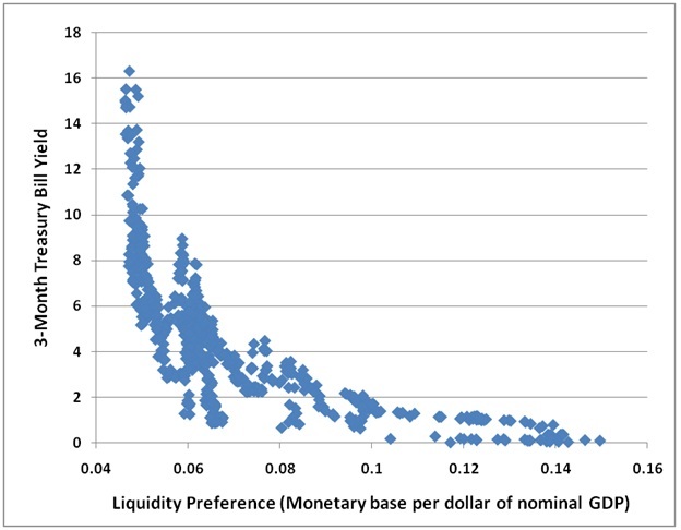
Sixteen Cents: Pushing the Unstable Limits of Monetary Policy

John P. Hussman, Ph.D.
All rights reserved and actively enforced.
Reprint Policy

This week's comment focuses on the current, unstable stance of monetary policy. We'll start by reviewing some important monetary relationships. While I've included a variety of graphs and equations to support the analysis, I've boldfaced several key points, and my hope is that the text has enough detail that you can skip some of the equations if you're not a math fan.

One of the best known relationships in economics is the concept of "liquidity preference" - essentially money demand. Both theoretically and in actual data, there is a fairly tight relationship between short-term interest rates, and the amount of non-interest-bearing money that people are willing to hold, either directly as currency, or indirectly as bank reserves. Basically, the lower interest rates are, the more cash or reserves ("base money") people are willing to carry around, per dollar of nominal GDP. As interest rates move higher, people naturally respond to the opportunity to earn interest by reducing the amount of cash they carry, both directly and indirectly.

You can see this relationship in the chart below, which plots the 3-month Treasury bill yield versus liquidity preference for base money. Though "liquidity preference" is often used to describe the broad demand for money, we will define liquidity preference more specifically here as the amount of base money demanded per dollar of nominal GDP. In post-war data, the lower bound for liquidity preference has been roughly 5 cents of base money holdings for every dollar of nominal GDP. With interest rates nearly zero at present, people are directly and indirectly holding much larger amounts of base money, currently slightly more than 13 cents for every dollar of GDP. The cluster of points at the extreme right of the graph are recent data. In a panic to hold cash, liquidity preference hit 15 cents at the height of the 2009 credit crisis.

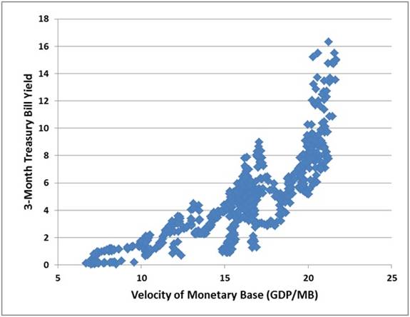
By comparison, Japanese liquidity preference has historically ranged from a low of about 0.08 to a high of nearly 0.12 when interest rates have been pressed toward zero.

The idea of monetary "velocity" seems slightly more theoretical, but velocity is simply the inverse of liquidity preference: it measures the amount of nominal GDP per dollar of monetary base. Not surprisingly, the chart of velocity is a mirror image of liquidity preference.

The exchange equation

OK. So we've established that there is a clear relationship between money demand and interest rates. As it happens, there's also a well-known relationship between money, velocity, output and prices, which is called the "exchange equation." The exchange equation is actually just a simple identity. Notice that nominal GDP is just real GDP ("Y") times the GDP price index ("P"). Velocity is equal to nominal GDP divided by the monetary base, so

V = PY/M

which is usually written

MV = PY

Although this is a simple identity, people like to tinker with one variable or another while incorrectly assuming that the other parts of the equation are simply constant. For example, people often assume that doubling the monetary base will simply double the price level, but that requires V and Y to stay constant, which is hardly an accurate assumption. Likewise, advocates of easy money seem to believe that increasing the money supply will buy you more economic output, but this requires holding V and P relatively constant.

If you look at the historical data, neither of these arguments hold a great deal of water. Rather, what seems to be true is that the strongest effect of an increase in the money supply is to drive short-term interest rates lower, thereby increasing liquidity preference (i.e. reducing velocity). So periods of very high growth in the monetary base are typically accompanied by nearly proportionate plunges in monetary velocity, without any strong effects on output or prices. As we'll see below, that isn't quite the whole story, but to a first approximation, the main effect of changes in the monetary base is to produce opposite and proportional changes in velocity.

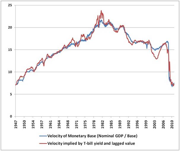
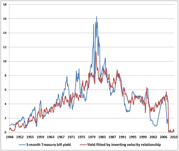
From this perspective, there is little reason to expect the Fed's policy of "quantitative easing" to have real effects on economic output. Thus far, quantitative easing has had the effect of increasing idle bank reserves by about $62 billion since September, with a slight downward impact on Treasury bill yields. On a seasonally-adjusted basis, the monetary base has increased by about $36 billion since September, but since the seasonal adjustment factor plunges in the first two months of the year as holiday cash demands subside, the seasonally-adjusted monetary base will spike by about $60 billion even if the Fed does nothing in the next two months.

Of course, QE2 has had additional effects on the financial markets, but these have not been driven by monetary factors. Instead, they are rhetorical, based on the view that somehow the Fed's actions create a "backstop" that will prevent potential losses in risky assets. As Ambrose Evans-Pritchard has noted, "the Fed no longer even denies that the purpose of its latest blast of bond purchases, or QE2, is to drive up Wall Street, perhaps because it has so signally failed to achieve its other purpose of driving down borrowing costs." Unfortunately, it is easy to demonstrate that the greater the volatility of a security or income stream, the smaller the "wealth effect" that can be expected from a given increase in value. Volatile dollars have less impact on consumption than smooth dollars, which is why housing values have historically had a much greater wealth effect than stock market values.

Moreover, people clearly believe that the additional reserves are flowing wildly into risk assets, pushing prices higher as if secondary markets are some sort of balloon to be filled (one second of reflection will establish that every dollar that goes "into" a secondary market in the hands of a buyer comes back "out" of the secondary market in the hands of a seller). The fact, however, is that these reserves are sitting comfortably in the banking system as idle balances.

As a study by the Bank of Japan of its own huge experiment with QE concluded, "While we can enumerate several routes of the monetary base channel which suggest that expansion of the monetary base can have some expansionary effect on the economy, our analyses suggest that the quantitative magnitude of any such effect is highly uncertain and very small." [The Effect of the Increase in the Monetary Base on Japan's Economy at Zero Interest Rates - An Emprical Analysis, Bank of Japan, 2002].

In any event, it is clear that with regard to risky securities, the enthusiasm and rhetoric about QE2 has caused a reduction in the willingness of sellers to sell, and an increase in the eagerness of buyers to buy. That imbalance of eagerness between buyers and sellers has clearly affected prices of risky assets, but it does not generate new cash flows - it simply raises the valuation that the market places on existing streams of future cash flows, and thereby lowers the subsequent rate of return on holding those securities. I suspect this will end badly, but that's not the topic of this discussion.

Quantifying monetary policy

So let's review. Liquidity preference is simply the amount of monetary base that people are willing to hold, per dollar of nominal GDP. We've seen that this demand for base money is essentially a function of short-term interest rates. When interest rates are low, people are willing to hold higher cash balances. When interest rates are high, people tend to economize on cash balances.

Just a note - even if you hate math, it will help to skim the next few paragraphs, but feel free to skip to the next graph if you wish. After inverting velocity, taking logarithms, and doing other calculations that geeks find entertaining, it turns out that the liquidity preference function can be estimated fairly accurately. Using the 3-month Treasury bill ("i") alone, the relationship in post-war data is well described* by:

M/PY = .094 - .022 * ln(i)

which gives you an implied equation for the 3-month Treasury bill yield as a function of liquidity preference:

i = exp(4.27 - 45.5*M/PY)

An even tighter relationship can be obtained by including the value of liquidity preference six months earlier:

M/PY = .0327 - .0077 * ln(i) + .65 * (M/PY)_lagged_6_mos

which again gives you an implied equation for the 3-month Treasury bill yield as a function of monetary variables:

i = exp(4.25 - 129.87*M/PY + 84.42*M/PY_lagged_6_mos)

The foregoing parameters are based on standard scaling factors used for reporting the variables, so GDP are and monetary base are in billions, and T-bill rates are in standard format. For example, given a current monetary base of $2,000 (billion) and nominal GDP of about $14,900 (billion), the expected 3-month Treasury bill yield here would be roughly exp(4.27-45.5*2000/14900) = 0.1592, which is about right (presently, the Treasury bill yield is 0.16%).

[* Geek's Note - The single variable version above is not estimated directly (there are better parameterizations possible if you want to "fit the curve" in a visually satisfying way). Rather, the estimate above is based on the "steady state" of the more accurate dynamic version. That is, if you set M/PY as a constant (steady state) in the dynamic version (which has an R^2 of about .96), you get M/PY = .0327 - .0077 * ln(i) + .65 * M/PY, which has the steady state of M/PY = .094 - .022 * ln(i). Using the dynamic version is more accurate for period-by-period estimates and for brief shifts in interest rates, but it won't immediately pick up the full effect of sustained interest rate changes unless you run the estimates forward to allow the lagged effects to kick in. For that reason, we'll use the steady state version below when we estimate responses to policy changes.]

Let's take a quick look at the fit from these estimates. The chart below shows the actual velocity of the monetary base, along with estimated velocity. Notice that we've observed an enormous plunge in velocity over the past two years, which is fully consistent with the near-zero level of interest rates at present.

Of course, we can also invert this relationship. The chart below shows the actual level of the 3-month Treasury bill yield, along with the yield implied by monetary variables.

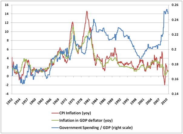
Pushing monetary policy to its unstable limits

But what about inflation? How is monetary policy related to prices?

Here is where things get really interesting. We've established that to a large extent, both liquidity preference and short-term interest rates respond fairly passively to changes in the monetary base. But of course, that's not the whole story. Not every change in interest rates or liquidity preference is passive, and when there is an exogenous "shock" to those factors - watch out.

Let's go back to the definition of liquidity preference (we'll call it "L").

L = M/PY

So

P = M/LY

It follows that we can impute the price level (GDP deflator) using base money, real GDP, and the level of liquidity preference implied by short-term interest rates.

With real GDP expected at about $13,409 billion in 2005 dollars for the fourth quarter of 2010, the implied GDP deflator is 2000/[(.094-.022*ln(.15))*13,409] = 1.10. The latest reading on the deflator was about 1.11, so the estimate is just about right.

The disturbing fact about this, however, is that inflation dynamics can potentially become unstable when a massive stock of base money is being kept in check by very low interest rates. This is because small increases in interest rates from near-zero levels imply huge changes in liquidity preference and velocity. If those changes are not offset by opposite and proportional changes in the monetary base, strong inflation pressures are likely to follow. Historically, it has usually taken an extended period of such inflation pressures (sustained over 6-12 months) before the implied inflation pressures are actually reflected in price levels. Temporary differences between the actual and implied GDP deflator are not very informative unless they are sustained.

Still, any sustained external pressure on short-term interest rates, even in the range of a quarter-percent or more, would require a rapid contraction in the Federal Reserve's balance sheet, or the upward pressure on velocity would create very strong incipient pressures on inflation.

For example, let's repeat the calculation for the implied GDP deflator, but assume a 3-month Treasury bill yield of 0.35%. In that case, holding the monetary base constant at its present level of $2 trillion, the implied deflator is 2000/[(.094-0.022*ln(0.35))*13,409] = 1.27. Compared with the 1.11 deflator implied by a 0.15% Treasury bill yield, the implied change in prices is about 14.4%.

Because the size of the monetary base has become so extreme relative to historical norms, the likely price pressures in response to even modestly higher short-term interest rates are equally extreme. For example, given the present level of the monetary base, an exogenous increase in short-term Treasury yields to even 1% would imply a GDP deflator of about 1.59, which is about 42.9% higher than present levels. In order to counter such pressure, the Fed would have to contract the monetary base by about $600 billion, from the present level of about $2 trillion to a still bloated but less extreme $1.4 trillion.

A larger increase in Treasury bill yields to 4% would imply a GDP deflator of about 2.35, which is more than double the current price level. The implication is that any normalization of interest rates would need to be accompanied by a massive contraction of the Fed's balance sheet in order to avoid inflation, otherwise the collapse in liquidity preference (resulting from the higher interest rates compared to zero interest on base money) would trigger a collapse in the purchasing power of cash.

The main factor that reduces the risk of massive inflation is that short-term interest rates usually respond fairly passively to changes in the monetary base. Also, while the Fed can do little to increase the returns to holding currency, it does have the ability to raise the interest rate that it currently pays banks to hold idle reserve balances, in order to keep those balances idle. So absent external pressures on short-term interest rates, the Fed may be able to continue playing at the edge of the proverbial cliff for a while longer.

Still, the absence of such pressures should not be taken as a given. Any external pressures on short-term interest rates would wreak havoc on the stability of monetary policy here. In the face of upward pressures on short-term interest rates, the Fed would have to contract the monetary base in an amount equal and opposite to the implied change in the deflator.

At the same time, barring external upward pressures on interest rates, a further non-inflationary expansion of the Fed's balance sheet of $400 billion, to $2.4 trillion (as contemplated under QE2), would imply the need for 3-month Treasury yields to fall to just 0.05%. Higher rates would be inflationary, because monetary velocity would not be sufficiently restrained. In effect, a further expansion in the monetary base requires that short-term interest rates decline enough to ensure a significant drop in velocity.

In terms of liquidity preference, a completion of QE2 requires liquidity preference to increase to 16 cents per dollar of nominal GDP - easily the highest level in history. We hit 15 cents at the peak of the credit crisis. To get past that, short-term interest rates will have to decline to the point where there is no competition from interest rates at all, but where the slightest amount of interest rate pressure would either drive inflation higher or force a massive contraction in the Fed's balance sheet to avoid that outcome. Then what?

Again, I should emphasize that even if we observe inflation pressures on the basis of the monetary relationships above, it typically takes an extended period of 6-12 months before those pressures become clearly reflected in price levels (so the relationship between actual and implied inflation is tighter if the data are smoothed over several quarters). In any event, it should be clear that the Fed is operating at an unstable extreme, and further expansion of the Fed's balance sheet will only increase that instability.

Present considerations

What factors could create pressures on inflation? By itself, monetary policy often involves a simple see-saw, where higher monetary base results in lower short-term interest rates, which induce people to hold that additional base money. Historically, both in the U.S. and internationally, the primary source of inflation pressure has been growth in unproductive government spending (i.e. spending that creates demand without materially expanding productive capacity - think Germany paying striking workers in the Ruhr). Now, it's very often true that government spending is actually financed by printing money, but in that case, we've long argued that the fiscal event is what drives inflation. Simply shifting the composition of government liabilities between Treasury debt and money (without changing fiscal policy) generally causes a change in the profile of interest rates: primarily affecting short-term rates to ensure that the new outstanding quantity of base money is held (as we've seen above).

While not all U.S. government spending is unproductive, it is easily seen that the inflation pressures of the late-1960's and 1970's accompanied a period where government spending was sharply expanding as a share of GDP (the 1981-82 recession provoked a final gasp of spending even as inflation receded from its peak). While the disinflation since the early 1980's has had some fits and starts, it is also clear that this period has - until recently - been characterized by relatively stable fiscal policy. From this perspective, the recent explosion of government spending as a share of GDP is a source of longer-term inflation concern.

With regard to the U.S. economy, we continue to observe some surface progress. Barring fresh shocks, our benchmark expectation (based on gradual reversion to potential GDP) would be for job growth averaging about 200,000 per month on a sustained basis, and real GDP growth of about 3.8% annually for several years before slowing. However, that proviso "barring fresh shocks" is my real concern. Nominal GDP may be recovering, but about 10% of that still represents deficit spending. The Fed's balance sheet, as noted here, stretches the limits of monetary policy - risking instability and a lack of robustness to small shocks.

As for the U.S. financial system - particularly major banks - I am continually perplexed by the juxtaposition of tens of millions of underwater mortgages and millions of delinquent and unforeclosed homes, coupled with a set of FASB accounting rules (revised at the height of the recent crisis) that allows these debts to be carried at face value upon the discretion of the banks that report the data. I'll say one thing - it should take less than two seconds of thought to recognize that allowing dividends, bonuses, and other withdrawals of capital - without the requirement that banks mark their assets to market - is quite literally how Ponzi schemes function. We've laid a lovely turf lawn over a toxic waste dump, and are all too willing to assume that the underlying issues have been solved. The FASB and the Fed have turned the U.S. banking system into the Love Canal.

In any event, completing the Fed's planned purchases under QE2 will require a decline in 3-month Treasury bill yields to just 0.05% in order to avoid inflationary pressure. Otherwise, liquidity preference will not expand sufficiently to absorb the addition to base money, even if we assume real GDP growth at a 4% rate. Given the extreme stance of monetary policy, the avoidance of inflationary pressures increasingly relies on a very persistent willingness by the public to directly or indirectly hold the outstanding quantity of base money in the financial system. Small errors will have surprisingly large consequences. This is not a stable equilibrium.

Market Climate

As of last week, the Market Climate for stocks remained characterized by an overvalued, overbought, overbullish, rising yields syndrome that has historically been very hostile for stocks, but is also accompanied by "unpleasant skew" - a tendency for the market to make a series of successive, marginal new highs, typically resolved by an abrupt plunge that wipes out weeks or months of upside progress in a few sessions. If you look at a chart, you can see this tendency for small, compressed daily ranges advancing to marginal new highs over the past several weeks. You'll see the same tendency at other periods that we've observed this syndrome, including memorable ones such as late 1972, August 1987, and numerous instances in more recent data, February 1997, April 1998 (though the final resolution in that case came several months later, it eventually wiped out all the interim gains and then 15% more), June 2007, January 2010, April 2010, and today.

Based on the broader set of Market Climates we define (see my comments on this over the past two months) we expect to establish moderate, if transitory, exposure to market fluctuations more frequently. That will likely include at least a moderately constructive investment stance (with a safety net around the mid-1100's) at the point where we clear some element of this syndrome, provided that internals don't also break down decidedly. Rather than "waiting" for whatever is going to happen to happen, we prefer to focus our efforts on aligning our investment positions with the prevailing Climate we observe in stocks, bonds, and precious metals. In stocks, that Climate is hard negative here and now, so Strategic Growth and Strategic International Equity remain fully hedged.

In bonds, the Market Climate last week was characterized by slightly unfavorable yield levels and increasingly unfavorable yield pressures. The Strategic Total Return Fund continued to have a relatively short duration of less than 2 years, exposing the Fund to little impact from interest rate fluctuations. In precious metals, the Market Climate improved, and we re-established a moderate (not aggressive) exposure to precious metals shares amounting to just under 8% of assets. While an aggressive exposure in precious metals most likely will require a reversal of long-term interest rate trends and some amount of fresh economic weakness, our focus is not so much on the next Market Climate we may observe next but on the Climate we observe at present.

A final note - next week's update will be very different than most. As you know, we've directed a great deal of effort in the past two years to "ensemble methods" and challenging problems involving the use of multiple data sets. While I expect that the benefits of applying this research in our investment approach will become clear over time, I'll be sharing the results we recently obtained by applying this line of research to a completely different sort of data - and a discovery that we hope will lead to improvements in the lives of hundreds of thousands of individuals.