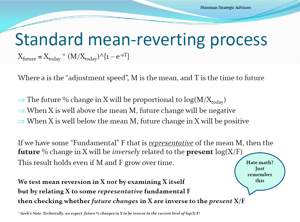
Two Point Three Sigmas Above the Norm

John P. Hussman, Ph.D.
All rights reserved and actively enforced.
Reprint Policy

“If you want to say that valuation measures are higher now, and that should be the norm, or that low interest rates now justify higher valuation measures, what you’re really saying is that long-term prospective returns should be lower, and they should be in the 2-3% annual range looking out a decade.”

– John Hussman, Very Mean Reversion, April 2014

While the S&P 500 Index is about 12% above April 2014 levels, my impression is that it may be surprising how quickly that gain is erased as the present cycle is completed. That initial erasure will likely be nothing but a very minor warm-up. At present, the most reliable measures we identify indicate that the S&P 500 is about 128% above the levels that would be historically associated with 10% long-term returns, and imply a net loss, including dividends, for the S&P 500 over the coming decade. Including a broader range of alternate (if slightly less reliable) measures brings that overvaluation to about 114% above historical norms, and results in our expectation of S&P 500 nominal total returns averaging just 1.5% annually over the coming decade.

I should emphasize that our total return projections embed the assumption of future growth in nominal GDP and S&P 500 revenues of 6% annually, despite the fact that these measures have grown at a rate of only 3.4% annually over the past 10-15 years. The reason we haven’t slashed our assumed growth rates is that historically, nominal growth and interest rate effects tend to cancel out in these projections. Specifically, if we get continued slow growth over the coming decade, we’re also likely to see depressed interest rates go hand-in-hand with that. The slower growth would negatively affect returns, but the lower interest rates could positively affect returns by encouraging somewhat higher terminal valuations. Historically, the 10-year Treasury yield has a positive correlation with nominal GDP and S&P revenue growth over the preceding decade, while stock valuations based on market cap/GDP or price/revenue have a negative correlation with nominal growth rates over the preceding decade. What we observe across a century of history is that those two effects repeatedly cancel out.

A brief primer on mean reversion

We see a great deal of misunderstanding about mean reversion in current financial discussions. Probably the most frequent error is the idea that one can determine whether or not market variables (such as valuation multiples or profit margins) are mean reverting simply by eyeing a chart or running a trendline through the data. As I discussed in my 2014 Wine Country Conference talk, Very Mean Reversion (which remains relevant to current market conditions), the correct test for mean reversion is to examine the relationship between present levels and subsequent changes in a given variable. 

For example, suppose F is some relatively smoothly growing fundamental that is a representative and sufficient statistic for the stream of long-term cash flows that stocks are expected to deliver to investors over time. Value investors would tend to believe that price is mean-reverting relative to F. The question is how one tests for that. The improper strategy is to simply examine a long-term chart or to run a trendline through the data. Why? For the same reason that one can’t determine that a sine wave is mean reverting by running a trendline from its low point to its high point. It may be that your data hasn’t captured the complete cycle.

Instead, the tipoff to mean reversion is to examine the relationship between the level of X/F and subsequent changes in X. In finance, we often think of X as price, the mean M as "fair value," and we look for fundamentals F that are essentially representative or proportional to fair value. The test for mean reversion is whether the ratio of Price/F (technically the logarithm of Price/F) is inversely related to actual subsequent price changes. If you were to look at a chart of valuations in 2000, an investor might have said "there is no way that this series is mean reverting." They would have been terribly wrong, and they could have known it at the time by understanding the distinction between eyeballing a chart and testing for a relationship between current level and subsequent changes.

We see the same problem when people look at profit margins. They run a trendline through the chart and say, "see, it slopes up" as if this is evidence that mean reversion doesn't exist. Again, this is just as improper as running a trendline through a sine wave regardless of the sample. The correct way to test for mean reversion is to test the relationship between current margins and subsequent profit growth. On that test, we continue to observe profit margins to be one of the most mean reverting series in finance, right next to valuations. When investors make the mistake of paying elevated price/earnings multiples on earnings that reflect elevated profit margins, very bad things happen - always have, always will.

Bonus for Geeks: The following is one of my slides from the WCC presentation last year. It gives a mathematical framework to think about mean reversion (and may help to understand why we often use logarithms when we estimate the relationship between valuations and subsequent returns). If you love math, you might recognize that the logarithm of the equation below also reduces to an Ornstein-Uhlenbeck process, which says xf = m + exp(-aT)(x0-m) and can easily handle negative values of x or m.

If you hate math, just understand that the proper way to test for mean reversion is to examine the relationship between your valuation multiple and actual subsequent market returns.

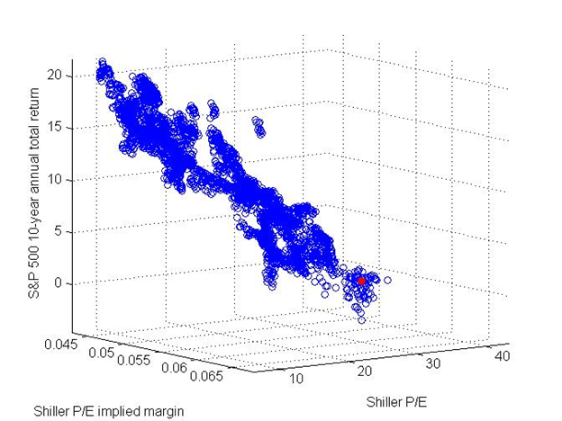
Let's make all of this more concrete by applying it to stock market valuations. Among non-proprietary measures of valuation we track, here are the correlations we presently estimate in post-war data between various valuation ratios and actual subsequent 10-year total nominal returns of the S&P 500:

log(price/trailing 12-month earnings): -0.76
log(price/forward operating earnings – data prior to 1980 imputed): -0.79
log(Shiller P/E): -0.83
log(Tobin’s Q: market cap/net worth at current cost): -0.85
log(Shiller P/E with adjustment for embedded profit margin): -0.88
log(nonfinancial market capitalization/nominal GDP): -0.88
log(price/revenue): -0.89

The reason for this perhaps odd-looking ranking of correlations is that while profits matter enormously in the sense that they are needed to generate deliverable cash flows, current profits – especially for the market as a whole – are also notoriously bad “sufficient statistics” for the long-term stream of those cash flows. That’s a direct result of the fact that profit margins are highly cyclical. The more a valuation measure flattens out those cyclical variations in profit margins, the more accurate the valuation measure is in projecting actual subsequent market returns. The ratio of market cap to nominal GDP and the price/revenue ratio dominate virtually all other valuation metrics in properly estimating long-term investment returns from stocks. We’ve discussed the minimal impact that foreign earnings have on these arguments in prior commentaries – see for example Do Foreign Earnings Explain Elevated Profit Margins? No.

Benjamin Graham, the father of value investing, advised investors to smooth out those cyclical variations by averaging profits over a number of years, which is the logic behind the Shiller P/E (the S&P 500 divided by the 10-year average of inflation-adjusted earnings). Some analysts have found that 16-year averaging improves on the measure (see What Does that Difference Mean?). Our own work indicates that the most reliable variant comes from adjusting the Shiller P/E explicitly for the embedded profit margin (see Margins, Multiples, and the Iron Law of Valuation). The following chart provides a nice illustration of how multiples and margins work together. The worst situation possible is when investors are paying elevated multiples on earnings that are already bloated by record profit margins. That is the situation in which we find ourselves today.

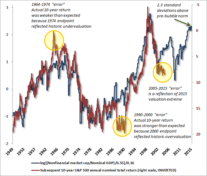
A similar observation extends to individual stocks, particularly those that have enjoyed unusual margin expansion or have unstable revenue bases. To quote Benjamin Graham, “Observation over many years has taught us that the chief losses to investors come from the purchase of low-quality securities at times of good business conditions. The purchasers view the good current earnings as equivalent to ‘earning power’ and assume that prosperity is equivalent to safety.”

Having reviewed other popular valuation measures, we should at least mention the Fed Model. If we correlate actual 10-year S&P 500 total returns with the Fed Model (forward operating earnings yield – 10 year Treasury yield), we should find a positive rather than negative correlation, since the Fed Model uses yields instead of multiples. Unfortunately, that correlation is only 0.48. The Fed Model does somewhat better in projecting the S&P 500 total return in excess of the 10-year Treasury yield, but then, A-X will almost always be correlated with B-X even if A and B have no relationship. As I observed at the 2007 top when the same measure was used to mislead investors about value, the Fed Model isn’t entirely useless, but it’s dominated by even the crudest alternatives available (see Long-Term Evidence on the Fed Model and Forward Operating P/E Ratios).

Two Point Three Sigmas Above the Norm

One of the things that may slightly comfort investors here is Jeremy Grantham’s recent observation that while the Shiller P/E and Tobin’s Q are 1.5 and 1.8 standard deviations above their long-term averages, respectively, they are not yet overvalued by “two sigmas.” Now, I respect Grantham more than virtually anyone else in the investment world, but I also believe that these figures understate current extremes for several reasons I’ll detail below. I’ll summarize our own assessment first. Based on the most reliable valuation measures we identify, stock market valuations are already 2.3 sigmas above reliable historical norms.

The following chart provides a good illustration of the present situation. The chart shows the ratio of market capitalization to GDP, which has a nearly 90% correlation with actual subsequent S&P 500 total returns over the following decade. I’ve presented the left scale in terms of standard deviations (see the section on mean reversion to understand why we take logarithms first). Actual subsequent total returns for the S&P 500 are shown by the red line, on an inverted right scale, so higher levels imply lower subsequent 10-year market returns.

In a 2001 Fortune article, Warren Buffett correctly identified market cap to GDP as “probably the best single measure of where valuations stand at any given moment.” While Buffett hasn’t mentioned this ratio in quite a while, it remains highly correlated with other historically reliable valuation measures. As we’ve seen throughout history, the transient “errors” in these measures are actually quite informative. Our valuation concerns certainly don’t rely on this particular metric, but it nicely summarizes the current situation.

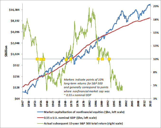
Why isn’t market/cap to GDP 100% correlated with subsequent 10-year market returns? The answer is that there are some 10-year periods in history where market valuation reached an extraordinary extreme at the end of that 10-year period. When that happens, the actual market return over that 10-year period will have been much higher or lower than one would have expected in advance, based on the level of starting valuations. The three most important examples are highlighted in the yellow circles.

In 1964, for example, valuations were about 1 standard deviation above the norm, so one would have expected below-average total returns of about 7% annually over the following decade. As it happened, however, 1974 marked the end of a 50% plunge in the market that took valuations to one of the lowest levels in the post-war period. As a result, actual 10-year returns were actually negative, and much weaker than expected for the 1964-1974 period. Investors were highly rewarded in the years following that valuation trough, particularly once the secular bear market ended in 1982.

Conversely, in 1990, the market was undervalued from the standpoint of historical norms, so one would have expected 10-year returns well above a run-of-the-mill 10% annual return. As it happened, though, the endpoint of that 10-year horizon was 2000 – the climax of the most extreme valuation bubble in history. As a result, actual 10-year returns from 1990-2000 were far higher than even the above-average returns one would have anticipated. Investors reaped the whirlwind in the plunge that followed.

Which brings us to the present, when the 2005-2015 total return of the market has been higher than one would have projected based on 2005 valuations. With current valuations 2.3 sigmas above the norm, it should be clear that this “error” is precisely the result of extreme valuations at present, and is highly informative about the risks that investors face ahead. While our baseline expectation for 10-year total returns is currently 1.5% on a broad range of measures, we should not be at all surprised if the actual total return ends up being negative. Market returns will only surprise to the upside over the coming decade to the extent that valuations fail to correct to levels that they’ve corrected to even in recent cycles – and neither of those declines have taken valuations anywhere near levels historically associated with secular undervaluation.

So why do we find a 2.3 sigma overvaluation while Grantham’s figures are in the 1.5-1.8 range? Two reasons. First, as noted above, the raw Shiller P/E and Tobin’s Q are historically dominated by other valuation measures, including the margin-adjusted Shiller P/E, market capitalization to GDP, and price/revenue. At present, the profit margin (Shiller earnings/current S&P 500 revenues) embedded into the Shiller multiple is currently about 6.8% versus a historical norm of just 5.4%. At normal margins, the Shiller multiple would not be 27 but 34. By contrast, the embedded margin at the March 2000 peak was 5.1%. At normal margins, the Shiller multiple would not have been 43 but 41. Valuations are currently much closer to the 2000 peak than the raw Shiller multiple would imply.

Second, when one calculates a standard deviation, one must first subtract out the average, and it’s here where one can quietly introduce a bias. Suppose, for example, that a healthy guinea pig weighs 32 ounces, but encounters an extreme illness where his weight drops to just 8 ounces for a prolonged period. Should we now take the average of those weights as the “norm” for the weight of a guinea pig? I think not. Rather, if we want our norm to mean something, we need to link it to some measure of health. Suppose that a healthy heartbeat for a guinea pig is 240 beats a minute, and that the heartbeat is tightly correlated with the weight of the animal. In that case, we should calibrate our norm to be the weight that is associated with a healthy rate of 240 beats per minute. Essentially, if we want to use the weight of the guinea pig as some indication of subsequent outcomes, we should measure deviations from the conditional mean - the normal weight of a guinea pig, conditional on the guinea pig not keeling over - not the unconditional mean.

Likewise, if we want a valuation norm to mean something, we should be attentive to the following question: what is the level of valuation that is associated with a reasonable “norm” for actual subsequent market returns? If one studies the data carefully across reliable valuation measures, it turns out that pre-bubble norms (i.e. data prior to the late-1990’s) are robustly associated with total market returns of about 10% annually. If we want our “sigmas” to mean something, we should use them to mean something consistent – the deviation from the valuation level that would normally be associated with historically run-of-the-mill total returns. That way, if we think that future returns should be lower than those historic norms, we can usefully say that a positive deviation is “justified.” At present, valuations are only justified if investors believe that stocks should achieve zero total return and zero risk premium whatsoever over the coming decade. We’re open to arguments that would contemplate a somewhat higher bias to valuations than we’ve seen historically, but as we also recognized in 2000 and 2007, the valuations we observe at present are ridiculous even in the context of current interest rates (see the discussion on interest rates and valuation in The Delusion of Perpetual Motion).

The following chart illustrates the “norm” concept. The blue line is nonfinancial market capitalization in $billions on a log scale. The pre-bubble norm for market capitalization to GDP is about 0.55 (the current ratio is about 1.32), so the red line tracks 0.55 times nominal GDP. The green line on the right scale shows the actual subsequent 15-year total return of the S&P 500 as a proxy for “long-term” returns. The yellow markers identify points where the S&P 500 actually went on to achieve an ordinary 10% long-term total return over that horizon. Notice that those markers correspond fairly well to points where the blue and red lines intersect. Put simply, the pre-bubble valuation norms of historically reliable valuation indicators do a fairly good job of identifying points where stocks were priced to achieve “run-of-the-mill” long-term returns of about 10% annually.

For our part, we think a decade is quite a long-time to assume away any event that would provoke investors to demand something close to a normal, run-of-the-mill 10% prospective market return at some point in that decade. Even in depressed interest rate environments, prospective equity returns tend to be weakly correlated with interest rates and rate movements (and are often negatively correlated). The only span in history where the correlation was clearly positive was during the inflation-disinflation cycle from the mid-1960’s to the mid-1990’s. If you’re waiting for stocks to become overvalued by 2 standard deviations, we’re already past that, and we would not be at all surprised to observe another decade of negative total returns on the S&P 500, as we observed the last time valuations were similar on the most reliable measures.

The enormous problem for investors here is that they have nowhere to hide. The absence of places to hide emphatically does not make the prospects for stocks any better – it simply means that conventional portfolios are likely to achieve total returns of next to nothing over the coming 8-10 years. At the 2000 extreme, large-capitalization stocks were breathtakingly overvalued, but 10-year Treasury bonds yielded 6.5%, and numerous smaller stocks were reasonably valued, especially on a relative basis. Presently, the price/revenue ratio of the median stock is at the highest level in history (see my friend Meb Faber’s post Stocks are the Most Expensive, Well, Ever). The outcome of yield-seeking speculation on the financial markets seems glorious in hindsight, precisely because security prices have been chased to untenable valuation extremes. The completion of this cycle is likely to be an equally extreme mirror image. 

The problem with extreme valuations is that once they emerge, there’s no way for investors, in aggregate, to avoid poor long-term returns or intermediate-term losses. It’s just an unfortunate situation because those outcomes are baked in the cake and somebody has to hold these securities over time. The only question is how the outcomes are distributed across investors. It may be best for those losses to be borne by the same investors who temporarily achieved paper gains, so we’re not keen on changing anyone’s mind to our point of view – it just means that someone else will take the hit.

Still, for those who trust our work, do think carefully about the likelihood of a stock market loss on the order of 50% over the completion of this cycle. That’s certainly less than the 83% loss that we correctly projected for tech stocks in 2000, but about the same that we warned for the S&P 500 in 2000. As market internals deteriorated, we elevated our valuation concerns to a crash warning in October 2000 and again in October 2007, which is again the situation that concerns us at present.

Learn this lesson during the bubble, or you’ll learn it during the crash: what distinguishes a bubble that continues higher from a bubble that crashes with little additional warning is the condition of investor risk preferences as inferred from market internals, credit spreads, and other risk-sensitive measures. I’ve learned that lesson twice in my investment career – once during the late-1990’s bubble when we adapted by introducing those measures of internals, and again in the recent half cycle since 2009 because the ensemble methods that emerged from our stress-testing against Depression-era data didn’t emphasize those features strongly enough (we ultimately imposed them as an overlay in mid-2014). Overvaluation always matters for long-term returns – it’s just that it only reliably matters over the shorter-run once market internals indicate a shift toward risk-aversion. At that point, overvaluation matters with a vengeance, though the precise timing can still be unpredictable and abrupt. That’s the risk we observe here. Our valuation concerns won’t vanish if market internals and credit spreads were to improve materially, but the immediacy of those concerns would be deferred.

Regardless of near-term conditions, recognize the risk of negative equity returns for a decade, as we projected in 2000 even under optimistic assumptions, and consider alternative assets and hedged vehicles more heavily here than you might if stocks were not overvalued, as was true in late-2008 (despite my later stress-testing inclinations that began our significant stumble in the recent half-cycle). Having completed and addressed that awkward transition in mid-2014, we’re more confident today than we’ve ever been in our methods, and my expectation is certainly that we’re well-prepared to navigate the coming cycle. Agree or disagree, we do believe that the present remains an ideal moment to align your portfolio with your actual tolerance for risk and your true investment horizon.

The foregoing comments represent the general investment analysis and economic views of the Advisor, and are provided solely for the purpose of information, instruction and discourse. Please see periodic remarks on the Fund Notes and Commentary page for discussion relating specifically to the Hussman Funds and the investment positions of the Funds.

---

The foregoing comments represent the general investment analysis and economic views of the Advisor, and are provided solely for the purpose of information, instruction and discourse.

Prospectuses for the Hussman Strategic Growth Fund, the Hussman Strategic Total Return Fund, the Hussman Strategic International Fund, and the Hussman Strategic Dividend Value Fund, as well as Fund reports and other information, are available by clicking "The Funds" menu button from any page of this website.

Estimates of prospective return and risk for equities, bonds, and other financial markets are forward-looking statements based the analysis and reasonable beliefs of Hussman Strategic Advisors. They are not a guarantee of future performance, and are not indicative of the prospective returns of any of the Hussman Funds. Actual returns may differ substantially from the estimates provided. Estimates of prospective long-term returns for the S&P 500 reflect our standard valuation methodology, focusing on the relationship between current market prices and earnings, dividends and other fundamentals, adjusted for variability over the economic cycle (see for example Investment, Speculation, Valuation, and Tinker Bell, The Likely Range of Market Returns in the Coming Decade and Valuing the S&P 500 Using Forward Operating Earnings ).