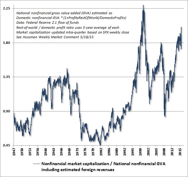
Rarefied Air: Valuations and Subsequent Market Returns

John P. Hussman, Ph.D.
All rights reserved and actively enforced.
Reprint Policy

The atmosphere is getting thin up here, and every ounce counts triple when you're climbing in rarefied air. While near-term market dynamics are more likely to be impacted by Friday’s employment report than any other factor, our broad view remains that stocks are in the late-stage top formation of the second most extreme episode of equity market overvaluation in U.S. history, second only to the 2000 peak, and already beyond the 1929, 1937, 1972, and 2007 episodes, not to mention lesser extremes across history.

On the economic front, much of the uncertainty about the current state of the economy can be resolved by distinguishing between leading indicators (such as new orders and order backlogs) and lagging indicators (such as employment). It’s not clear whether the weakness we’ve observed for some time in leading indicators will make its way to the employment figures in time to derail a Fed rate hike in December, but as we’ve demonstrated before, the market response to both overvaluation and Fed actions is highly dependent on the state of market internals at the time. Presently, we observe significant divergence and internal deterioration on that front. If we were to observe shift back to uniformly favorable internals and narrowing credit spreads, our immediate concerns would ease significantly, even if longer-term risks would remain.

Having reviewed the divergences we observe across leading economic indicators and market internals last week (see Dispersion Dynamics), a few additional notes on current valuations may be useful.

As I’ve noted before, the valuation measures that have the strongest and most reliable correlation with actual subsequent market returns across history are those that mute the impact of cyclical variations in profit margins. If one examines the deviation of various valuation measures from their historical norms, those deviations are rarely eliminated within a span of a year or two, but are regularly eliminated within 10-12 years (the autocorrelation profile drops to zero at that point). As a result, even the best valuation measures have little relationship to near-term returns, but provide strong information about subsequent market returns on a 10-12 year horizon. Among the most reliable valuation measures we identify, those with the strongest relationship with subsequent 12-year nominal S&P 500 total returns are:

Shiller P/E: -84.7% correlation with actual subsequent 12-year S&P 500 total returns
Tobin’s Q: -84.6% correlation
Nonfinancial market capitalization/GDP: -87.6%
Margin-adjusted forward operating P/E (see my 8/20/10 weekly comment): -90.7%
Margin-adjusted CAPE (see my 5/05/14 weekly comment): -90.7%
Nonfinancial market capitalization/GVA (see my 5/18/15 weekly comment): -91.9%

MarketCap/GVA is presented below to provide a variety of perspectives on current valuation extremes. The first chart shows this measure since 1947. We know by the relationship between MarketCap/GVA and other measures (with records preceding the Depression) that the current level of overvaluation would easily exceed those of 1929 and 1937, making the present the most extreme point of stock market overvaluation in history with the exception of 2000. In hindsight, the only portion of 2000 when stocks were still in a bull market was during the first quarter of that year.

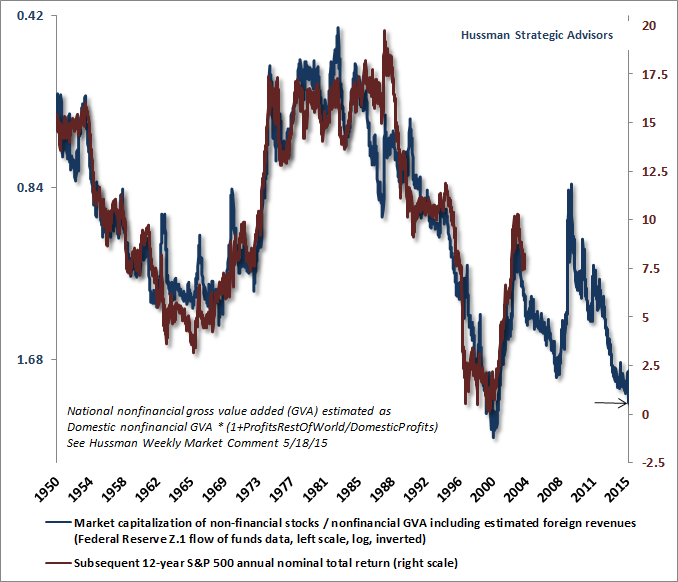
To be as clear as possible: Over the near term, broad improvement in market internals and credit spreads would suggest a return to risk-seeking speculation that might defer the unwinding of this obscene Fed-induced speculative bubble, or could even extend it. But with market internals presently negative and credit spreads continuing to widen, the market remains vulnerable to an air-pocket, panic or crash, here and now. In either case, our expectation is that the completion of the current market cycle will involve a market loss of at least 40-55%; a loss that would merely take the most historically reliable valuation measures to run-of-the-mill pre-bubble norms, not materially below them.

Investors should remember from the 2000-2002 and 2007-2009 collapses that in the absence of investor risk-seeking - as conveyed by market internals - even aggressive Fed easing does not support stocks. The reason is that once investors become risk-averse, safe, low-interest liquidity is a desirable asset rather than an inferior one. So creating more liquidity fails to achieve what the Fed does so successfully and perniciously during a risk-seeking bubble: drive investors to chase yield and speculate in risk-assets.

I should be the first to point out my own errors in the recent bubble, and the central lesson to be drawn. In market cycles across history, the emergence of extreme overvalued, overbought, overbullish conditions was typically either accompanied or closely followed by a deterioration in market internals (signaling that investors had shifted to risk aversion), and market collapses followed in short order. I responded to the emergence of those syndromes directly by taking a hard-defensive outlook. If the Federal Reserve’s unprecedented recklessness did one thing in this cycle, it was to disrupt that overlap; extreme overvalued, overbought, overbullish conditions were followed by further speculation rather than any shift toward risk-aversion among investors. One had to wait until market internals had explicitly deteriorated before taking a hard-defensive market outlook. We imposed that requirement on our discipline in mid-2014.

If you’re not familiar with this narrative, see The Hinge. We know exactly what we got wrong in this half-cycle, exactly how we’ve addressed it, and exactly how those adaptations would have performed across a century of market history, including the most recent cycle. That historically-informed perspective is the basis for our confidence here. In contrast, many speculators seem to have no clue that they are about to experience the same consequences that followed the 2000 and 2007 speculative extremes. They’ve learned no lesson from either, so they’ll have to live through similar outcomes again.

The chart below places MarketCap/GVA on an inverted log scale (blue line, left scale), along with the actual S&P 500 nominal annual total return over the following 12-year period (red line, right scale). Note that current valuations imply a 12-year total return of only about 1% annually. Given that all of this return is likely to come from dividends, current valuations also support the expectation that the S&P 500 Index will be lower 12 years from now than it is today. While that outcome may seem preposterous, recall that the same outcome was also realized in the 12-year period following the 2000 peak.

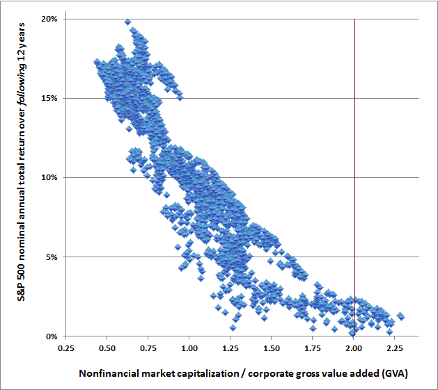
The following scatter plot shows the data in a slightly different way, but to the same effect.

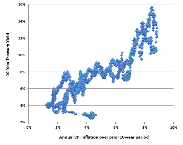
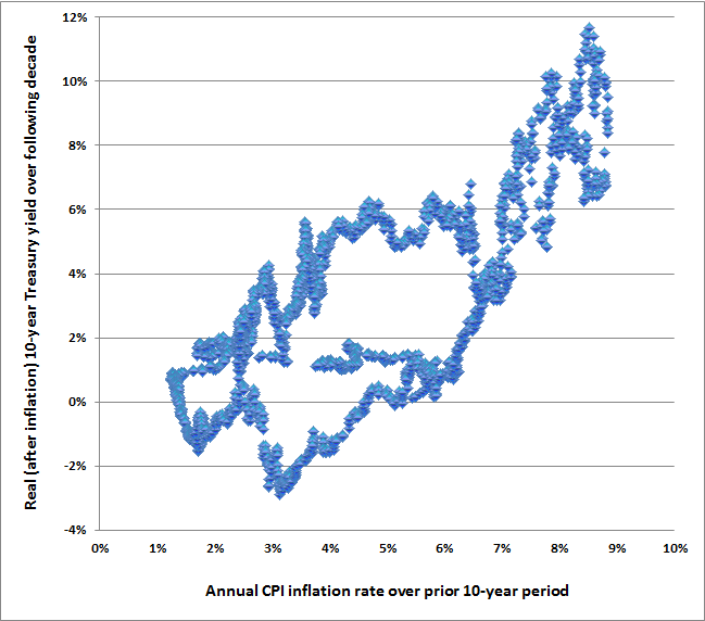
Valuations and returns; real and nominal

One of the questions we’re periodically asked is why we use equity valuation measures to project nominal returns rather than real returns. In theory, a higher level of inflation should raise the growth rate of fundamentals, but should also increase the required rate of return on a security, resulting in a valuation ratio that is actually independent of inflation. In that kind of “Fisher-effect” world, any change in equity valuations would correspond to a change in expected real returns, not nominal ones, because the impact of inflation would wash out of the calculation.

In order for that to hold, the requirement is that expected nominal stock returns (i.e. the discount rate applied to future cash flows) and nominal growth in fundamentals must be identically impacted by inflation, so that stock valuation multiples remain independent of inflation. One can show this using a discounted cash flow approach. For any security - stocks or bonds - if investors respond to inflation by changing the discount rate in a way that’s not identical to the change in the future growth rate of fundamentals, there will not be a one-to-one relationship between the valuation multiple and the subsequent real return.

As the simplest example, consider a Treasury bond: since the cash flows are fixed, any change in the valuation “multiple” (e.g. bond price/coupon payment) must represent a change in the discount rate alone. As a result, changes in valuation are perfectly correlated with subsequent nominal returns.

How closely do U.S. financial markets resemble a perfect Fisher-effect world? Let’s take a look at data since 1947. One of our first expectations would be that interest rates should respond to changes in expected inflation. It’s not surprising at all that 10-year Treasury yields are strongly related to the rate of inflation over the prior decade.

In a nice, Fisher-effect world, however, nominal interest rates would respond to past inflation just enough to compensate for likely future inflation, leaving expected real future Treasury returns unchanged. In practice, investors tend to respond much more strongly, and as a result, high past inflation tends to be followed by high real returns, not just high nominal returns. Likewise, low past inflation tends to be followed by low real returns, not just low nominal ones.

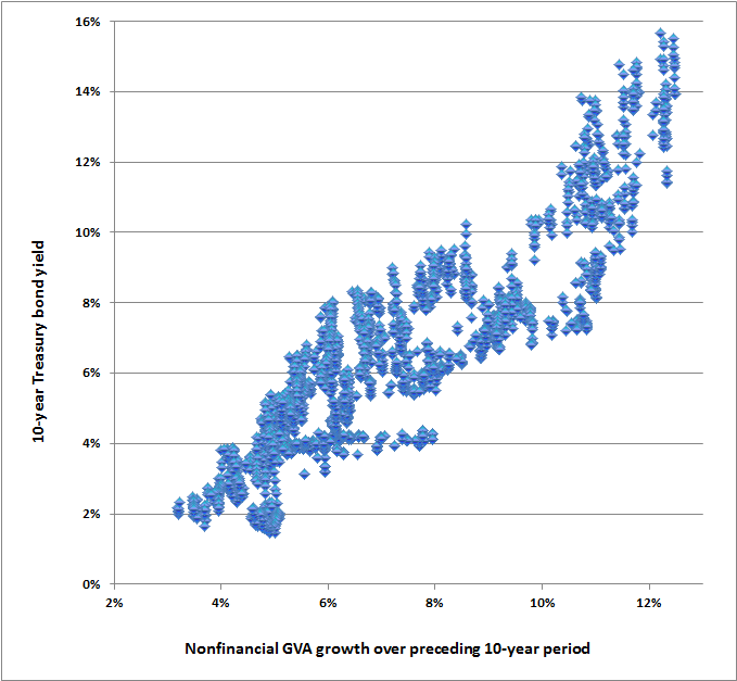
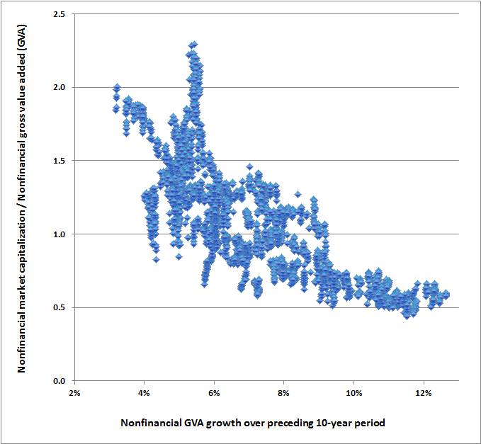
The same regularity extends not only to inflation, but nominal economic variables like gross domestic product. Since we’ve been using MarketCap/GVA as our preferred valuation metric, we’ll continue with that measure here. Notice first that there is a very strong positive relationship the 10-year Treasury bond yield and the nominal growth rate of corporate gross value added over preceding decade.

Stop and think about this chart for a moment. Many investors like to assume that interest rates will still be low a decade from now, thinking that this would support higher end-of-decade valuations for stocks and avoid poor market returns in the interim. Unfortunately, the only reason one would assume that interest rates will remain as low as they are now is if growth in the economy, revenues, GVA and other fundamentals turns out to be dismal over the coming years. In that event, low interest rates might support higher terminal valuation multiples for stocks, but on much lower fundamentals than otherwise. Across history, these effects of growth rates and terminal valuation multiples systematically wash out.

As it happens, neither past nominal nor real growth in GVA is well-correlated with nominal or real growth over the subsequent 10-year period. Variations in nominal growth over the past decade affect discount rates more than they affect the expected future growth of cash flows. As a result, more rapid nominal growth in the past tends to be associated with lower stock valuations, while slower nominal growth in the past tends to be associated (though not quite as reliably) with higher stock valuations.

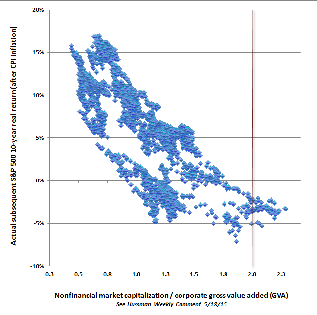
In summary, investors across history have systematically responded to high rates of inflation and past growth by driving up bond yields and driving down equity valuations, to the point where subsequent real and nominal investment returns have been quite strong. Conversely, investors have systematically responded to low rates of inflation and past growth by driving down bond yields and driving up equity valuations, to the point where subsequent real and nominal growth have been extremely poor.

The main instance when this inverse relationship between prior growth and terminal valuations did not hold as tightly was during the Depression and its aftermath. During that period, investors became conditioned to expect dismal economic growth, and responded by awarding the stock market with lower terminal multiples than they did in the post-war period. As a result, between 1926 and 1940, actual subsequent 10-year market returns ended up being weaker than one would have projected on the basis of post-war valuation relationships. Given the current environment of persistently sub-par economic growth, if there’s a risk to our projection of near-zero total returns in the S&P 500 over the coming 10-12 years, it’s likely that our expectations will turn out to be too optimistic.

Allow me just two minutes to formalize some of this. Remember how valuations, growth rates and investment returns are related. In the two equations below (skip over them if they send you into math panic) P is price, V is the valuation ratio of price to some fundamental, and g is the nominal growth rate of that fundamental over the following T years. We can then write the future capital gain precisely as:

P_future / P_today = (1+g)^T x (V_future / V_today)

Or in log terms:

log(P_future/P_today) = T x log(1+g) + log(V_future) - log(V_today)

All this says is that your future investment return is positively affected by: the holding period T, the growth of fundamentals g (assuming that growth is positive), and the future valuation multiple. In contrast, your future return is negatively affected by the current valuation multiple. Because departures of valuations and nominal growth from their historical norms tend to mean-revert over time, one can obtain reliable estimates of prospective 10-12 year market returns by using historical norms for g and V_future (see Ockham’s Razor and the Market Cycle for an illustration using a variety of valuation measures).

What may be less obvious is that those market return estimates are just as accurate even when actual growth and terminal valuations depart from their historical norms. Go back to the previous scatterplots, and you’ll notice something. The terminal valuation multiple is inversely related to nominal growth over the preceding decade, meaning that variations in the first two terms (from their historical norms) tend to offset each other. This isn’t random - it’s systematic. The reason, again, is that investors respond to high rates of inflation and past nominal growth by driving interest rates higher and equity valuations lower. Conversely, they respond to low rates of inflation and past nominal growth by driving interest rates lower and equity valuations higher (partly due to the kind of yield-seeking speculation we’ve seen in recent years).

What remains? A nearly direct inverse relationship between current equity valuations and subsequent nominal returns in market cycles across history. You can see that inverse relationship in the second graph of this weekly comment, which plots the log of MarketCap/GVA on an inverted scale, versus actual subsequent 12-year S&P 500 nominal total returns.

Q.E.D.

A quick side note. I generally ignore anonymous critics - open debate can be constructive, and provides a chance to learn from others, but my impression is that unless one is defending human rights in a politically hostile climate (where writing under pseudonym has worthy precedents), using anonymity as a veil to criticize others reflects the kind of intellectual cowardice that makes mice of men. Still, the foregoing may address the suggestion that the relationship between valuations and subsequent market returns is mere coincidence or curve-fitting. It should also be evident that the inverse (and generally offsetting) relationship between nominal growth and end-of-period valuations is quite systematic. If one wishes to imagine a parallel universe where these regularities don’t exist, and to dismiss the historical relationship between valuations and actual subsequent equity market returns across a century of data on that basis, by all means, be my guest.

Finally, it’s worth making clear that the relationship between reliable equity valuation measures and subsequent real returns is also significant. The red line on the chart below shows the current level of valuations. As the chart indicates, investors should presently expect unambiguously negative real returns in the S&P 500 over the coming decade from current valuation extremes.

As usual, investors who follow a passive buy-and-hold discipline, who don’t believe that valuations have meaningful implications for subsequent market returns, who would experience distress over missing potential market gains regardless of the valuation extremes in which they occur, who have carefully considered the actual depth of losses that the stock market has regularly experienced over the completion of market cycles, and who have aligned their investment exposure consistent with their actual investment horizon and risk tolerance - these investors can reasonably do nothing here, and we don’t at all encourage them to deviate from their discipline. Investors who could not reasonably tolerate a loss in the S&P 500 on the order of 50% (as the market has experienced in prior cycles), or who would abandon their discipline in that event, should recognize that such a loss is actually the run-of-the-mill expectation from current valuations.

The foregoing comments represent the general investment analysis and economic views of the Advisor, and are provided solely for the purpose of information, instruction and discourse. Please see periodic remarks on the Fund Notes and Commentary page for discussion relating specifically to the Hussman Funds and the investment positions of the Funds.

---

The foregoing comments represent the general investment analysis and economic views of the Advisor, and are provided solely for the purpose of information, instruction and discourse.

Prospectuses for the Hussman Strategic Growth Fund, the Hussman Strategic Total Return Fund, the Hussman Strategic International Fund, and the Hussman Strategic Dividend Value Fund, as well as Fund reports and other information, are available by clicking "The Funds" menu button from any page of this website.

Estimates of prospective return and risk for equities, bonds, and other financial markets are forward-looking statements based the analysis and reasonable beliefs of Hussman Strategic Advisors. They are not a guarantee of future performance, and are not indicative of the prospective returns of any of the Hussman Funds. Actual returns may differ substantially from the estimates provided. Estimates of prospective long-term returns for the S&P 500 reflect our standard valuation methodology, focusing on the relationship between current market prices and earnings, dividends and other fundamentals, adjusted for variability over the economic cycle (see for example Investment, Speculation, Valuation, and Tinker Bell, The Likely Range of Market Returns in the Coming Decade and Valuing the S&P 500 Using Forward Operating Earnings ).